What’s the Problem?

For quite awhile I was wondering about a potential disconnect in the way the Central Limit Theorem (a.k.a CLT) is taught and how it’s applied. Usually in statistics textbooks and online tutorials the reasoning goes like this:

• Step 1: Collect a set of observations (say, 20) and calculate the mean of that one sample of data
• Step 2: Collect another set of 20 observations and calculate the mean of that second sample of data
• Step 3: Repeat this process many, many times (say 10,000 times)
• Step 4: You now have 10,000 sample means. Plot a histogram of those sample means. (This is known as a distribution of sample means)
• Shazam! That distribution you plotted looks something like a normal distribution! That’s the CLT!

If you were to increase the set of observations collected each time from 20 to, say 25, then the resulting histogram would look even closer to a normal distribution.

This gives the impression it’s through repeatedly gathering sets of 20 (or 25 or more) observations we can say the distribution of the sample means is approximately normal. Boston University’s School of Public Health makes similar remarks:

The central limit theorem states that if you…take sufficiently large random samples from the population…then the distribution of the sample means will be approximately normally distributed

But what happens when you’re given only one sample of data? This is ordinarily the case in textbook examples and in real life, as there isn’t often enough money or time to collect more than one sample. How come we can invoke the CLT here? An example Boston University provides does just that, remarking

probability questions about a sample mean can be addressed with the Central Limit Theorem, as long as the sample size is sufficiently large

I bolded “sample mean” because we shifted from talking about a distribution of sample means (plural) to just a sample mean (singular)

This has proved confusing for a number of people, myself included, as is evidenced in this and this post from CrossValidated.

A Sweet Diversion

Suppose you want to find the average amount of m&m’s in share size bags. Obviously you can’t get all share size bags on the market, so instead you buy 50 bags and meticulously count the number of m&m’s in each bag, which inevitably differs from bag to bag.

From the thousands (if not millions) of share bags on the market (the population of m&m share bags), you obtained one sample of 50 bags. Suppose the mean amount of m&m’s in your sample turns out to be 29 and the standard deviation 5.

The sample mean (29) and sample variance (\(5^{2} = 25\)) of m&m’s are fantastic estimates (a.k.a unbiased estimators) of the population mean and population variance. So how can we use the sample we obtained to make inferences about the population mean of m&m’s in share bags? This is where the CLT comes in.

What the CLT really says

The CLT first and foremost tells us about the distribution of a sample average. We don’t need to know anything about the population itself. This is great since first, we only care about inferences on the mean, and second it can be painstakingly difficult or impossible to know everything about the entire population. Remember, we can’t buy all the m&m’s on the market!

So what can we say about the distribution of the sample average (or mean) of m&m’s we found? The CLT tells us:

• the shape of the distribution is approximately normal so long as the sample size \(({n})\) is at least 30
• the mean of the distribution is equal to the mean of the population distribution
• the variance of the distribution is smaller than the variance of the population distribution by a factor of \({1/n}\)

We can demonstrate this the hard way by working through the proof of the CLT, or by using simulation - which is much more intuitive and understandable. A great walk-through of such a simulation can be found in this Khan Academy video.

The CLT does not require having multiple samples, as these two notable statisitics textbooks demonstrate^{1 2}. Rather, drawing multiple samples through simulation is a way to see that the CLT makes sense.

Back to m&m’s

With these facts let’s return to the m&m’s example. Our sample size is 50, clearly greater than the requirement of 30, so we can apply the CLT. Our sample mean is 29 and our sample variance is 5. The distribution of the sample mean of share bag m&m’s enables us to make inferences about the population mean of share bag m&m’s.

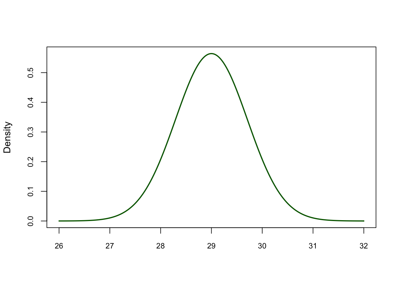
What does the distribution of the sample mean look like? It’ll look normally distributed with a mean of \(29\) and a variance of \(25/50 = 1/2\)

set.seed(3000)
xseq <-seq(26,32,.01)
densities<-dnorm(xseq, mean=29, sd=sqrt(25/50))
plot(xseq, densities, col="darkgreen",xlab="", 
     ylab="Density", type="l",lwd=2, cex=2, main="", cex.axis=.8)

This can tell us a lot of things! For example, there’s only a 0.23% chance of finding 31 or more m&m’s in a share bag.

pnorm(31, mean = 29, sd = sqrt(25/50), lower.tail = F)
## [1] 0.002338867

Conclusion

The main takeaway is the CLT enables us to derive the distribution of a sample mean from a just a single sample. You can use simulation to show that repeatedly obtaining samples will produce a distribution of the sample mean like the one shown for m&m’s above. Repeated sampling itself, though, has nothing to do with the CLT or its application.