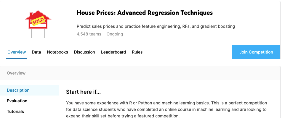
The venerable House Price Competition on Kaggle
In the graduate statistics class I’ve TA’ed, we explore a range of regression concepts, both theory and practice. This includes linear and polynomial regression, as well as transformations to align data to certain regression modeling assumptions. At the end of the course, students complete form groups to work on a project…the Kaggle housing prices competition on Ames, Iowa - perhaps the most well known and ongoing competition. This introduces students to real-world modeling and the ‘Kagglesphere’. Yes, we know linear regression isn’t the winning technique for this competition, but it’s simply an exercise in modeling. Also, the students in the best-scoring group gets 3 points extra credit on the final exam. That’s the real competition!
Before delving into building a full model on the entire dataset, students are given an “appetizer” (ok, it’s not actually called that but that’s how I refer to it) where they focus on predicting house selling prices for just three neighborhoods — Brookside, Edwards, and North Ames — using a home’s living area as a predictor. By using this smaller subset it’s easier to explore the effects of certain regression techniques, and interpret model output. After all, linear regression is a highly interpretable machine learning algorithm (yes, linear regression is machine learning) and should thus be exploited whenever possible.
Now, just because linear regression models are interpretable doesn’t mean they can’t become complex. Complexity often arises from combining use of interaction terms and logarithmic transforms. In the appetizer, interaction terms allow the slope of each neighborhood’s selling price to differ.
Suppose increasing a house’s living area is generally associated with an increase in a house’s price. An interaction term stipulates that the price hike per square foot increase of living area will be different for each of the three neighborhoods. A 1\({ft^2}\) increase in living area may be associated with a $50 increase in selling price for North Ames homes, a $30 increase for Brookside homes, and a $65 increase for Edwards homes.
Throwing in a log transform makes things a bit more tricky to interpret. Small wonder my textbook admonishes
“it is often difficult to interpret individual coefficients in an interaction model.”1
Several students came to me asking how to interpret interaction terms in a log-log model. I created a PowerPoint that became the basis for this blog post!
Log-Log Model with Interaction Terms
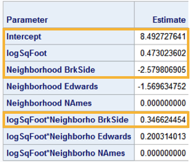
What would such a model look like for the appetizer model? Here’s some SAS output with the relevant portions highlighted

Notice that North Ames (NAmes) is considered the reference category. There’s no particular reason North Ames was chosen. We’ll focus on comparing Brookside home prices to North Ames prices. Our goal is to interpret logSqFoot*Neighborho BrkSide, the interaction term for Brookside homes.
Let’s first begin by writing out the equation for those neighborhoods (I’m rounding all values to the nearest hundredth).
Brookside
\(ln(Price) = 8.49+0.47*ln(sqft)-2.58+0.35*ln(sqft) = 5.91+0.82*ln(sqft)\)
North Ames
\(ln(Price) = 8.49+0.47*ln(sqft)\)
Notice how both the response and explanatory variables are (natural) log transformed.
Individual Interpretation
Generally speaking, an equation of the form \(ln(Y) = \beta_0 + \beta_1*ln(X)\) has the following interpretation:
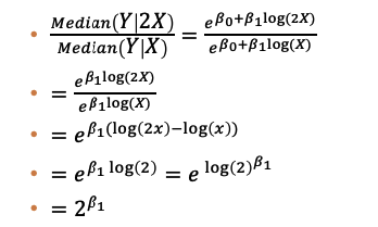
a doubling of X is associated with a \(2^{\beta_1}\) multiplicative increase in the median of Y
We can show this with the following derivation (taken from my class notes)

Applying this to our two equations above
Brookside Interpretation
A doubling in living area is associated with a \(2^{0.82}\) multiplicative increase (or 77% increase) in median Brookside home prices.
North Ames Interpretation
A doubling in living area is associated with a \(2^{0.47}\) multiplicative increase (or 39% increase) in median North Ames home prices.
Interaction Term Interpretation
Notice the interaction term logSqFoot*Neighborho BrkSide is 0.35, which is the difference between 0.82 and 0.47. This tells us 0.35 is the adjustment in the slope of home selling prices for Brookside homes, relative to North Ames homes. We can, however, give a more precise interpretation of the interaction term by noting
\(\frac{Multiplicative\,Increase\,BkSide}{Multiplicative\,Increase\,NAmes} = \frac{2^{\,0.82}}{2^{\,0.47}} = 2^{\,0.82-0.47} = 2^{\,0.35}\)
This implies
\(Multiplicative\,Increase\,BkSide = 2^{0.35}*(Multiplicative\,Increase\,NAmes)\)
So we can then say:
For a doubling in living area, the multiplicative increase in median sale price for Brookside homes is \(2^{0.35}\) (= 1.27) times greater than the multiplicative increase in median sales prices for North Ames homes, holding all other variables constant
Not a straightforward interpretation!
Motivating an alternate interpretation
Another way to interpret \(\beta_1\) in the equation \(ln(Y) = \beta_0 + \beta_1*ln(X)\) is
A 1% increase in X is associated with a \(\beta_1\)% increase in Y, holding all other variables constant
I’ll point you to this and this Stack Exchange post on why that makes sense. Those resources however don’t provide an interpretation of log-log interaction terms using percents. So let’s do that now.
Brookside Interpretation (with Percents)
A 1% increase in living area is associated with a 0.82% increase in median Brookside home price, holding all other variables constant
North Ames Interpretation (with Percents)
A 1% increase in living area is associated with a 0.47% increase in median North Ames home price, holding all other variables constant
This implies the following interpretation for logSqFoot*Neighborho BrkSide
There’s a 0.35 percentage point difference in median sales price between Brookside and North Ames homes for a 1% increase in living area, holding all other variables constant.
Note that going from 0.47% to 0.82% is a difference of 0.35 percentage points (not percent). In terms of a percent, it’s a \(\frac{0.82-0.47}{0.47}*100\) = 74.47% increase.
Interaction Interpretation Template
We can summarize both interpretations by providing a general template, where the terms in curly braces are replaced with the relevant variable names
“Doubling” Interpretation
For a doubling in {x-variable}, the multiplicative increase in median {response variable} for {category} is \(2^{interaction\,term\,value}\) times greater than the multiplicative increase in median {response variable} for {reference category}, holding all other variables constant.
“Percentage Point” Interpretation
There’s a {interaction term value} percentage point difference in median {response variable} between {category} and {reference category} for a 1% increase in {x-variable}, holding all other variables constant.
Wrapping Up
Perhaps it’s best to follow my textbook’s advice and avoid interpreting complex interaction terms. But if you’re a curious soul seeking meaning (of interaction terms), I hope this satisfies your curiosity.
The Statistical Sleuth, 3rd Edition (2013), Fred Ramsey and Daniel Schafer, p.250↩