Introduction
I love to bike, especially during the spring and summer. As a New York City resident the city affords miles of urban bike paths, my favorite being the seamless connection between Riverside and Hudson River parks. Of course thousands (if not millions) of others enjoy biking throughout the country, and if you don’t own a bike you can rent one through various bike programs, like NYC’s Citi Bike and Washington DC’s Capital BikeShare (CB henceforth). The latter is the focus of this report.
Background and Motivation
CB has maintained ridership data since 2010, but I first came across their data on the UCI Machine Learning Repository here which featured data from 2011-2012. A more complete analysis of CB’s ridership requires more data, so UCI’s data will be merged with 2013-2017 data from CB’s website.
The objective is to create 30-day trip forecasts by comparing several competing time series models. This task is relevant to CB officials since they could predict how much revenue to expect for any 30 day period. While location-based data isn’t utilized in this analysis, using it could help identify areas needing increased bike availability. And although daily data is used here, hourly forecasts would enable cyclists to gauge and anticipate future bike demand.
Literature Review
Bike share programs are relatively new, but research on factors affecting ridership has been conducted. Buck and Buehler 2011 have conducted research on CB ridership at the station level during CB’s first six months of operation. Using stepwise multiple regression model, they conclude average daily ridership is affected by the number of bike lines within 1/2 mile of a station, the number of Washington DC Alcohol Beverage Regulation Administration (ABRA) license holders, and the weighted average percentage of households with no access to an automobile (adjusted \(R^2\) = 0.66, n=91).
Rixey 2012 investigates the natural logarithm of monthly bike rentals across three bike share programs (including CB) from the first operating season of each, on a station basis using multiple regression. Rixey reduces his 19 candidate variables to 11 (plus an intercept) that include various socioeconomic and bike system architecture variables, yielding an adjusted \(R^2\) of ~0.8.
El-Assi, et al 2017 perform a similar types of analysis of Toronto’s bike share program, developing models for weekday, weekend, station origin, and station destination ridership. Adjusted \({R^2}\) values hover around 0.66.
Wang et al 2012 use 19 total socioeconomic variables to develop a regression model for station level, 2011 ridership of the Nice Ride bike share program in Minneapolis. Notably no weather variables are included. They achieve an adjusted Adjusted \({R^2}\) of approximately 0.87.
All of that research focuses more on identifying important variables and trends for ridership but not forecasting (extrapolating) future ridership. That is the focus of this analysis. It’s important to note high \(R^2\) values don’t necessarily translate into accurate forecasts since models can overfit the data. That issue was not examined in their analyses, so it’s unsure how predictive their models are. However, the variables they used may be helpful additions to this analysis (at some later date).
Data Cleaning and Feature Engineering
Data comes from three sources: UCI 2011-2012 data, historical weather data from NOAA for 2011-2017, and the CB ridership data from 2013-2017. We’ll go through each one; as the code is sufficiently commented, summaries of the data wrangling should suffice.
UCI Data (2011-2012)
We begin with the UCI data since it’s the quickest and serves as the baseline for how the remainder of data from 2013-2017 is handled.
Relevant revisions include:
- removing unnecessary weather and calendar variables - they’ll be replaced later on with other variables
- converting relevant calendar variables into factor/categorical variables
- converting weather data to their original, non-normalized scales
- adding a week of the month column. This isn’t completely necessary now, but it’s used later to define/encode holiday dates in the 2013-2017 data
# main libraries used; others will be loaded later
library(tswge)
library(fpp2)
library(lubridate)
library(dplyr)

############## Begin with UCI data ##############
# import 2011 and 2012 UCI data - will be merged with 2013-2017 data later
# change file path to match yours!
bikes_uci <- read.csv("day.csv")
# remove atemp since it adds no info on top of temp
# remove season and yr - unnecessary calendar variables
# remove instant; remove workingday - weekday covers this
# remove weathersit - cumbersome to define; this is replaced with actual rain and snowfall data
bikes_uci <- bikes_uci[, -c(1,3,4,8,9,11)]
# rename dteday to TripDate
colnames(bikes_uci)[1] <- "TripDate"
# add 1 to weekday to make consistent with everyday understanding (1-7)
bikes_uci$weekday <- bikes_uci$weekday+1
# convert calendar variables to factor variables
bikes_uci[, 2:4] <- lapply(bikes_uci[, 2:4], factor)
# convert date column to ymd format
bikes_uci$TripDate <- ymd(bikes_uci$TripDate)
# add weekofmon (needed later for the other years' holiday calculations)
bikes_uci <- bikes_uci %>%
  mutate(weekofmon = ifelse(between(day(TripDate),1,7), 1,
                            ifelse(between(day(TripDate),8,14), 2,
                                   ifelse(between(day(TripDate),15,21), 3, 4))))
# un-normalize temp; normalization formula: (t-t_min)/(t_max-t_min); t_max = 39, t_min=-8
bikes_uci$temp <- 47*bikes_uci$temp - 8
# convert temp from celcius to farenheit
bikes_uci$temp <- bikes_uci$temp * 9/5 + 32
# un-normalize humidity; normalization formula: hum/100
bikes_uci$hum <- 100*bikes_uci$hum
# convert weekofmon to factor
bikes_uci$weekofmon <- as.factor(bikes_uci$weekofmon)NOAA Historical Weather Data (2011-2017)
CB doesn’t include weather related variables like UCI does (the data contributor(s) added them separately), so we need to find this ourselves. It’s a fair assumption that temperature and precipitation affect ridership patterns so this is well worth finding. The data is included in my repository but here’s how you can get it yourself:
2) under Local Climatological Data, select “Search Tool”
3) choose State, then Virginia
5) click Add to Cart
6) go to your cart in the upper right hand side of the webpage; click View All Items
7) choose LCD CSV, select dates 2011-01-01 to 2017-12-31, then click Continue
8) fill in your email to get the data, then click Submit Order
The data will take a couple of minutes to be sent to your email
We’re only concerned with the date, temperature, precipitation, snow, wind speed, and humidity. Everything else can be discarded.
After examining the data we see December 31 info is missing for 2011, 2013 and 2014 so these are searched manually from timeanddate, averaging the four six-hour interval values for the aforementioned weather variables (data is given for 12am, 6am, 12pm, and 6pm). Precipitation and snow values denoted as T (trace amounts) are replaced with 0.
####### ---------- Include (dry-bulb) temperature, humidity, and precipitation data -------------###
# change file path to match yours
dc_weather <- read.csv("dcweather.csv")
# non-blank temps represent daily averages
dc_weather <- filter(dc_weather, !is.na(DailyAverageDryBulbTemperature))
# keep date, temp, and humidity columns - find their column numbers first
cols_keep <- match(c("DATE","DailyAverageDryBulbTemperature","DailyAverageRelativeHumidity",
                     "DailyAverageWindSpeed", "DailyPrecipitation", "DailySnowfall"),
                   colnames(dc_weather))
# remove everything else
dc_weather <- dc_weather[, cols_keep]
# shorten/rename columns
colnames(dc_weather) <- c("TripDate", "temp", "hum", "windspeed", "prec", "snow")
# remove "T" and time values from date column; first convert to character
# equivalent to keeping elements 1-10 of the date string
dc_weather$TripDate <- as.character(dc_weather$TripDate)
dc_weather$TripDate <- substring(dc_weather$TripDate,1,10)
# now convert TripDate column to TripDate object
dc_weather$TripDate <- ymd(dc_weather$TripDate)
# quick check of weather data (using summary function) reveals
# T values in prec and snow; T means trace amounts, so we'll substitute 0 for T
# info taken from https://www1.ncdc.noaa.gov/pub/data/cdo/documentation/GHCND_documentation.pdf
# first need to convert from factor to character - can't directly substitute from factor
dc_weather[, 5:6] <- apply(dc_weather[, 5:6], 2, function(x) as.character(x))
# now make the substitution
for (i in 5:6) {
  # if any value in column i equals T, replace with 0, otherwise keep original value
  dc_weather[, i] <- ifelse(dc_weather[, i] == "T", "0", dc_weather[, i])
}
# change prec and snow columns to numeric type
dc_weather[, 5:6] <- apply(dc_weather[, 5:6], 2, function(x) as.numeric(x))
# missing 12/31 date for 2011, 2013, and 2014. insert rows into dc_weather
# find row number Dec 30 for '11, '13, and '14.
dec_30s <- which(month(dc_weather$TripDate) == 12 &
                 day(dc_weather$TripDate) == 30 &
                 year(dc_weather$TripDate) %in% c(2011,2013,2014))

# create a small dataframe to hold Dec 31 info
dec_31_info <- data.frame(TripDate = ymd(c("2011/12/31", "2013/12/31", "2014/12/31")),
                          temp = c(58,41,36),
                          hum = c(62,49,43),
                          windspeed = c(9,11,7),
                          prec = c(0,0,0),
                          snow = c(0,0,0)
)

# cut and paste together all the weather data
dc_weather <- rbind(dc_weather[1:364, ], # 1/1/2011 - 12/30/2011
                     dec_31_info[1,], # 12/31/2011
                     dc_weather[365:1094, ], # 1/1/2012 - 12/30/2013
                     dec_31_info[2, ], # 12/31/2013
                     dc_weather[1095:1458, ], # 1/1/2014 - 12/30/14
                     dec_31_info[3,], # 12/31/14
                     dc_weather[1459:2919, ] # everything else
                     )
Combining all three datasets
Finally, we unite all three datasets to obtain 2011-2017 ridership data. First, we replace the deleted UCI weather data with the 2011-2012 info from NOAA. Then we update the CB data by attaching the NOAA weather data from 2013-2017 to it. Finally, we horizontally stack the UCI and CB data (2011-2012 on top, 2013-2017 on the bottom) to make one complete dataset called bikes.
############## combining all three datasets ##############
# add prec and snow values for 2011 and 2012 to bikes_uci
# these are the substitutes for weathersit
bikes_uci <- dc_weather %>%
  filter(between(TripDate, "2011/01/01", "2012/12/31")) %>%
  select(TripDate, prec, snow) %>%
  merge(bikes_uci, by="TripDate", all=T)

# merge dc_weather and cyclists -- this adds on the weather data to cyclists
bikes_temp <- merge(cyclists, dc_weather, by="TripDate")
# now we have all 2013-2017 data.  need to combine this with UCI 2011-2012 data
# first need to reorder columns of bikes_uci (or bike_temp)
cols_matched <- match(colnames(bikes_temp), colnames(bikes_uci))
bikes_uci <- bikes_uci[, cols_matched]
# now merge horizontally (stack UCI data on top of 2013-2017)
bikes <- bind_rows(bikes_uci, bikes_temp)
Final Data Cleaning
Curiously, all humidity data from October 2013 is missing (as well as for four other dates).
bikes[which(is.na(bikes$hum)), c(1,4,9:11)] TripDate cnt temp hum windspeed
1005 2013-10-01 10255 72 NA 5.0
1006 2013-10-02 10249 76 NA 5.8
1007 2013-10-03 10059 76 NA 4.3
1008 2013-10-04 10158 78 NA 3.2
1009 2013-10-05 10456 79 NA 4.6
1010 2013-10-06 9650 80 NA 8.8
1011 2013-10-07 5797 68 NA 12.3
1012 2013-10-08 9829 62 NA 8.2
1013 2013-10-09 6360 60 NA 12.7
1014 2013-10-10 2491 58 NA 13.4
1015 2013-10-11 1775 62 NA 11.0
1016 2013-10-12 5191 66 NA 11.2
1017 2013-10-13 5938 63 NA 10.8
1018 2013-10-14 8818 64 NA 6.7
1019 2013-10-15 9272 64 NA 3.6
1020 2013-10-16 9629 68 NA 4.9
1021 2013-10-17 9468 70 NA 7.7
1022 2013-10-18 10256 61 NA 6.6
1023 2013-10-19 9309 60 NA 6.9
1024 2013-10-20 8493 58 NA 8.7
1025 2013-10-21 8956 57 NA 7.1
1026 2013-10-22 8990 60 NA 7.3
1027 2013-10-23 7884 54 NA 8.0
1028 2013-10-24 7823 48 NA 9.0
1029 2013-10-25 7866 48 NA 8.9
1030 2013-10-26 7906 46 NA 10.1
1031 2013-10-27 7917 53 NA 5.5
1032 2013-10-28 8515 55 NA 3.3
1033 2013-10-29 8949 55 NA 2.7
1034 2013-10-30 8055 59 NA 3.6
1035 2013-10-31 8335 62 NA 8.1
1520 2015-02-28 3222 27 NA 5.1
2013 2016-07-09 12198 86 NA 8.4
2157 2016-11-30 6170 61 NA 6.0
2247 2017-02-28 7828 58 NA 4.9Fortunately we can use past values to impute missing data. The ACF plot below quantifies how strong current and past humidity values are correlated, such as ~ 0.5 correlation between a given day’s value and yesterday’s value.
Acf(bikes$hum, lag.max = 30, main="")
rect(xleft=0.5, ybottom=0, xright=1.5, ytop=0.53, border="red",lwd=2)
arrows(x0=4, y0=0.45, x1=2, y1=0.45, angle=20, col="red", length=.1)
text(x=3.7, y=0.45, labels = c("Lag 1"), pos=4, cex=.85)
title("Humidity Autocorrelations", line=1)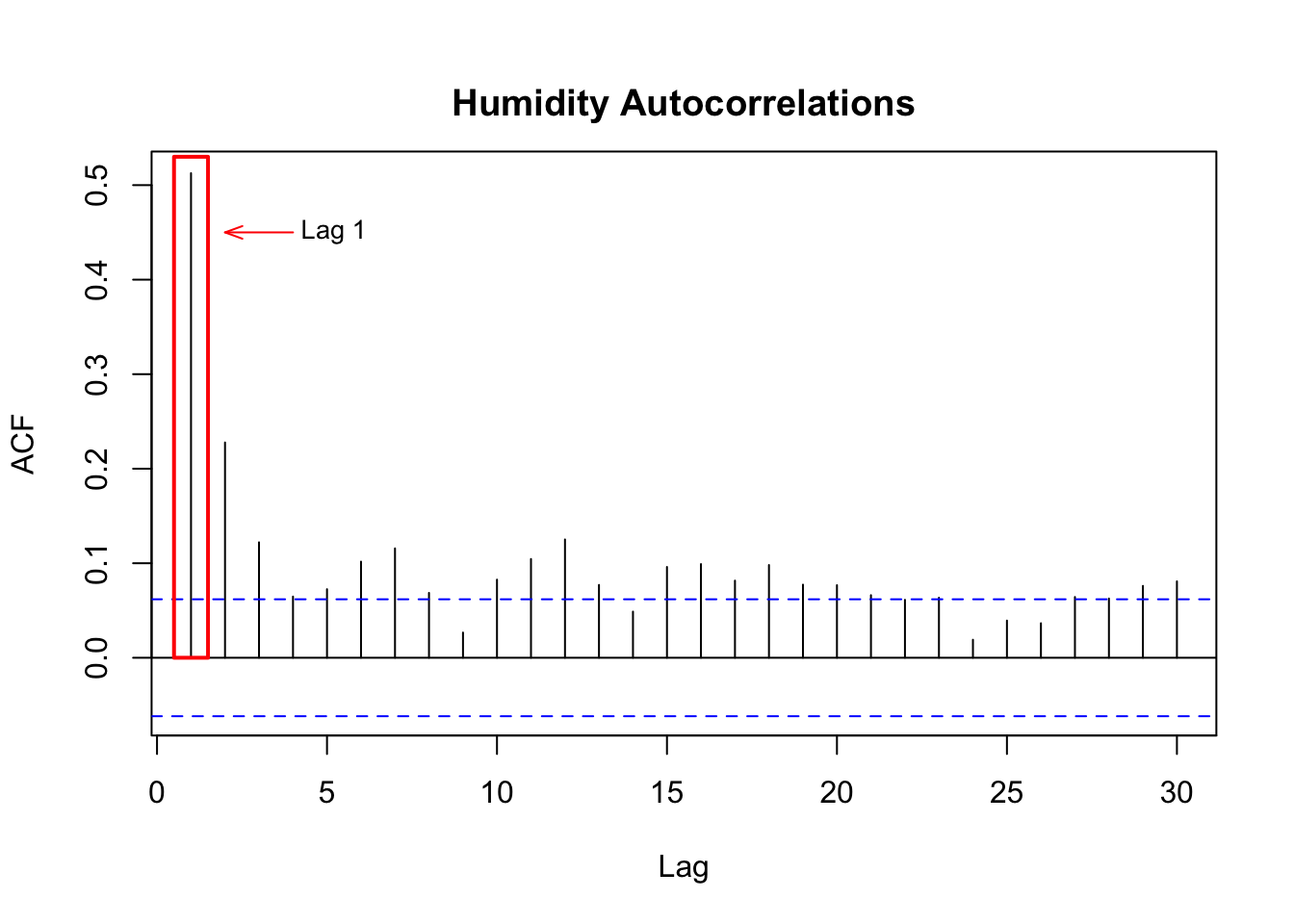
Using one day previous values of humidity would be great if we weren’t missing 31 consecutive days! However, if we assign a seasonality of 365 to humidity, decomposing the humidity data displays a strong annual pattern, as seen in the seasonal component below.
# remove NAs from humidity column
hum_2 <- na.omit(bikes$hum)
# make into ts object
hum_2_ts <- ts(hum_2, frequency = 365)
stl(hum_2_ts, s.window = "periodic") %>% autoplot() + xlab("Time (Years)") + theme_minimal()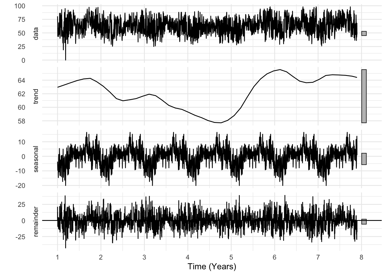
So we resort to using last year’s date ( ~ 365 days) for each missing date since there’s evidence of annual seasonality. For example, we’ll use humidity from 10/12/2012 as a substitute for 10/12/2013. It’s quite natural to ask what last year’s value of something was if you’re missing this year’s data and have evidence of annual seasonality, as we do here.
############## final data cleaning ##############
# find date of missing hum values and get the previous year's date
last_yrs <- bikes[which(is.na(bikes$hum)), ]$TripDate - years(1)
# get the associated humidity values
last_hum <- bikes %>%
  filter(TripDate %in% last_yrs) %>%
  select(TripDate, hum)
# impute by first storing relevant row numbers
rows_to_impute <- which(is.na(bikes$hum))
bikes[rows_to_impute, 10] <- last_hum$hum
# to model trend (in MLR model), need to include time variable (Time)
# Time is simply the length of the time series (1:nrow(bikes))
bikes$Time <- 1:nrow(bikes)
Lastly, we create a variable named Time which ranges from 1 to the total number of rows in bikes 2553, which implies Day 1 through 2553 of the dataset. Later on we’ll use this to model trend in our regression models.
Summary
There’s a lot in this section! It reflects how many data science analyses go: 70-80% of time is spent data cleaning and feature engineering, and there’s even more of the latter later in the modeling stage as we improve model performance. For now let’s restate what we’ve done so far.
- Replace categorical weather info in the UCI dataset with numerical values of snow and precipitation from NOAA
- Introduce week of month as an auxiliary feature, and use it alongside month of year to define federal holiday as a feature in the 2013-2017 data
- Impute missing weather data missing from NOAA
- Introduce a time variable to model trend (later in the analysis)
At this point we can (finally) explore the data!
Exploratory Analysis
Data Dictionary
Before exploring, here’s a summary of all the variables and their meanings.
library(kableExtra)
bike_variables <- data.frame(Variable = c("TripDate", "casual", "registered", "cnt", "weekday", "mnth", "weekofmon", "holiday", "temp", "hum", "windspeed", "prec", "snow", "Time"),
                             Description = c("Date of record", "Number of trips made by lower-tier membership plan riders", "Number of trips made by upper-tier membership plan riders", "Sum of the two previous columns", "Day of the week. 1 = Sunday", "Month of TripDate (1-12)", "Week of month of the TripDate (1-4)", "Is the TripDate a federal holiday? 1 = Yes", "Temperature in Fahrenheit", "Humidity expressed as a percent (maximum possible = 100)","Wind speed in miles per hour", "Amount of precipitation (rain) in inches","Amount of snowfall in inches", "Day Number (Day 1, Day 2, etc).  Used to model trend in regression models"))

bike_variables %>% kable() %>% kable_styling(full_width = F, bootstrap_options = "striped")| Variable | Description |
|---|---|
| TripDate | Date of record |
| casual | Number of trips made by lower-tier membership plan riders |
| registered | Number of trips made by upper-tier membership plan riders |
| cnt | Sum of the two previous columns |
| weekday | Day of the week. 1 = Sunday |
| mnth | Month of TripDate (1-12) |
| weekofmon | Week of month of the TripDate (1-4) |
| holiday | Is the TripDate a federal holiday? 1 = Yes |
| temp | Temperature in Fahrenheit |
| hum | Humidity expressed as a percent (maximum possible = 100) |
| windspeed | Wind speed in miles per hour |
| prec | Amount of precipitation (rain) in inches |
| snow | Amount of snowfall in inches |
| Time | Day Number (Day 1, Day 2, etc). Used to model trend in regression models |
Our variable of interest to predict is cnt.
Overall Daily Ridership
The line plot below is interactive, so feel free to click and drag around your mouse to zoom in on any portion. We see a clear positive trend and annual seasonality in ridership – for example, people tend to ride more during the summer than winter months.
The tall upward peaks in 2014 and 2015 most likely reflect high turnout at the annual National Cherry Blossom Festival.
ggplot(bikes, aes(TripDate,cnt)) +
  geom_line(col="steelblue") +
  xlab("")+
  ylab("Total Trips")+
  scale_x_date(breaks = "11 months") +
  ggtitle("Capital BikeShare Daily Trips (2011-2017)") +
  theme(panel.grid = element_blank(),
        plot.title = element_text(hjust=0.5, family = "Georgia"))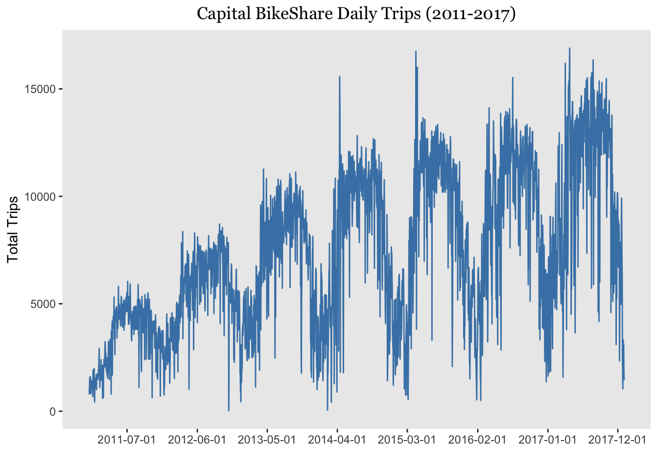
Exploring Weather Variables on Ridership
Below is a scatterplot matrix of continuous predictors (weather variables) plotted against each other and the response variable cnt (total number of trips). Some comments:
- No significant multicollinearity exists between the weather variables. This means regression coefficients for those variables should be stable
- Only temperature is strongly correlated with trip numbers
- Snowfall and precipitation negatively affect trips (as expected)
pairs(bikes[, c(4,9:13)], lower.panel = NULL, col="steelblue")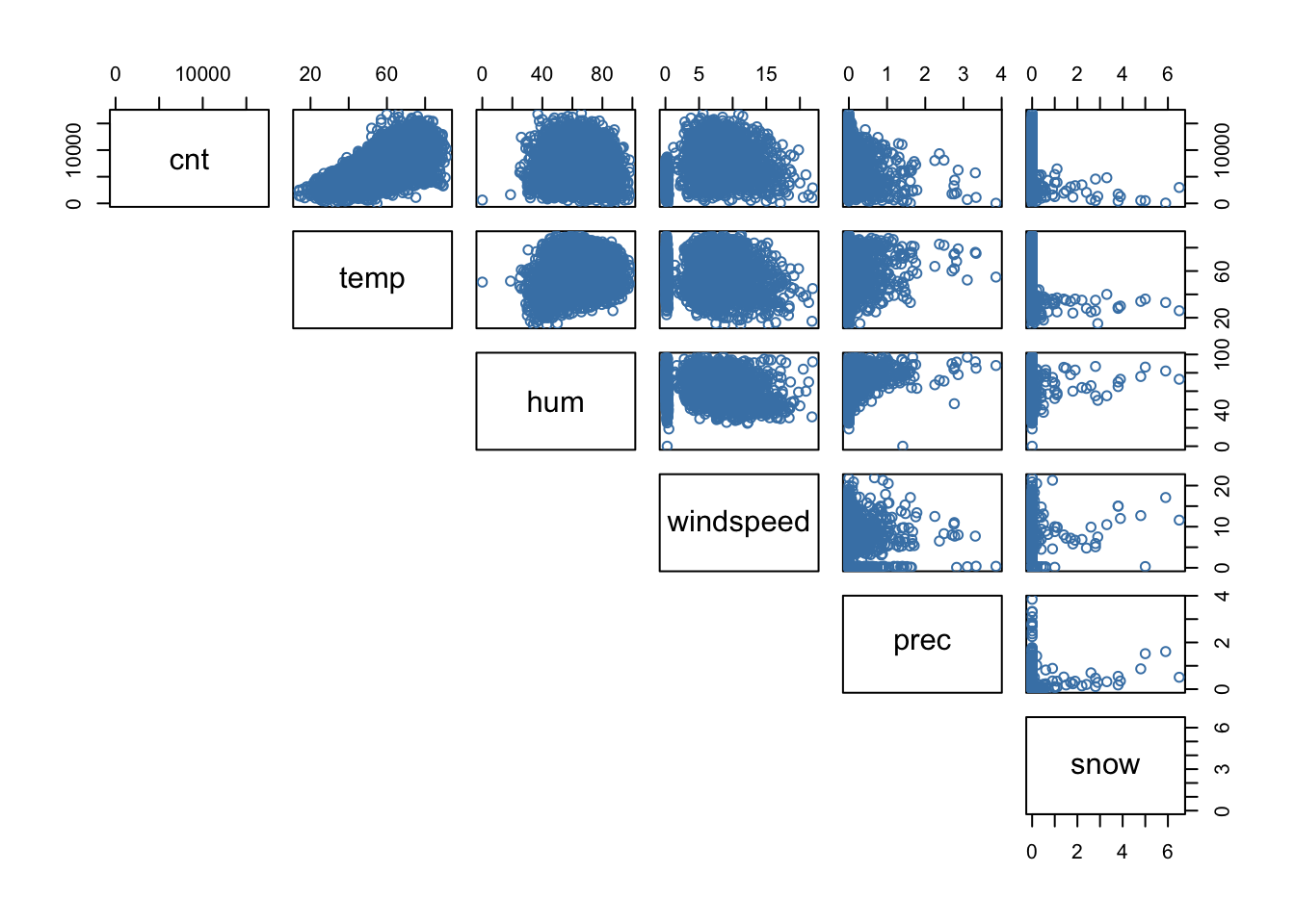
Ridership by Day of the Week
Trip patterns tend to fluctuate depending on day of week though not in a drastic way. Nevertheless people tend to ride more in the middle of the week (Wednesdays in particular, beginning in 2015) and less during the weekends.
library(numform)
library(gganimate)
library(magick)
dow_animation <- bikes %>%
  group_by(weekday, Year = as.integer(year(TripDate))) %>%
  summarise(`Total Trips` = sum(cnt)) %>%
  ggplot(aes(weekday, `Total Trips`)) +
  geom_bar(stat = "identity", fill="lightblue") +
  #geom_text(aes(label=paste0(round(`Total Trips`/1000), "K")), vjust=1.6, size=3.5)+
  scale_x_discrete(labels = c("1"="Sun", "2"="Mon", "3"="Tue","4"="Wed","5"="Thur","6"="Fri","7"="Sat"))+
  scale_y_continuous(label=ff_thous(digits=2))+
  theme(panel.background = element_blank(),
        axis.ticks = element_blank()) +
  labs(title="Total Trips by Day of Week: {frame_time}",
       x = "", y="Total Trips (in thousands)")+
  transition_time(Year)

dow_anim <- animate(dow_animation, nframes = 50, renderer = magick_renderer())
# save as gif
anim_save("dayofweek.gif", dow_anim)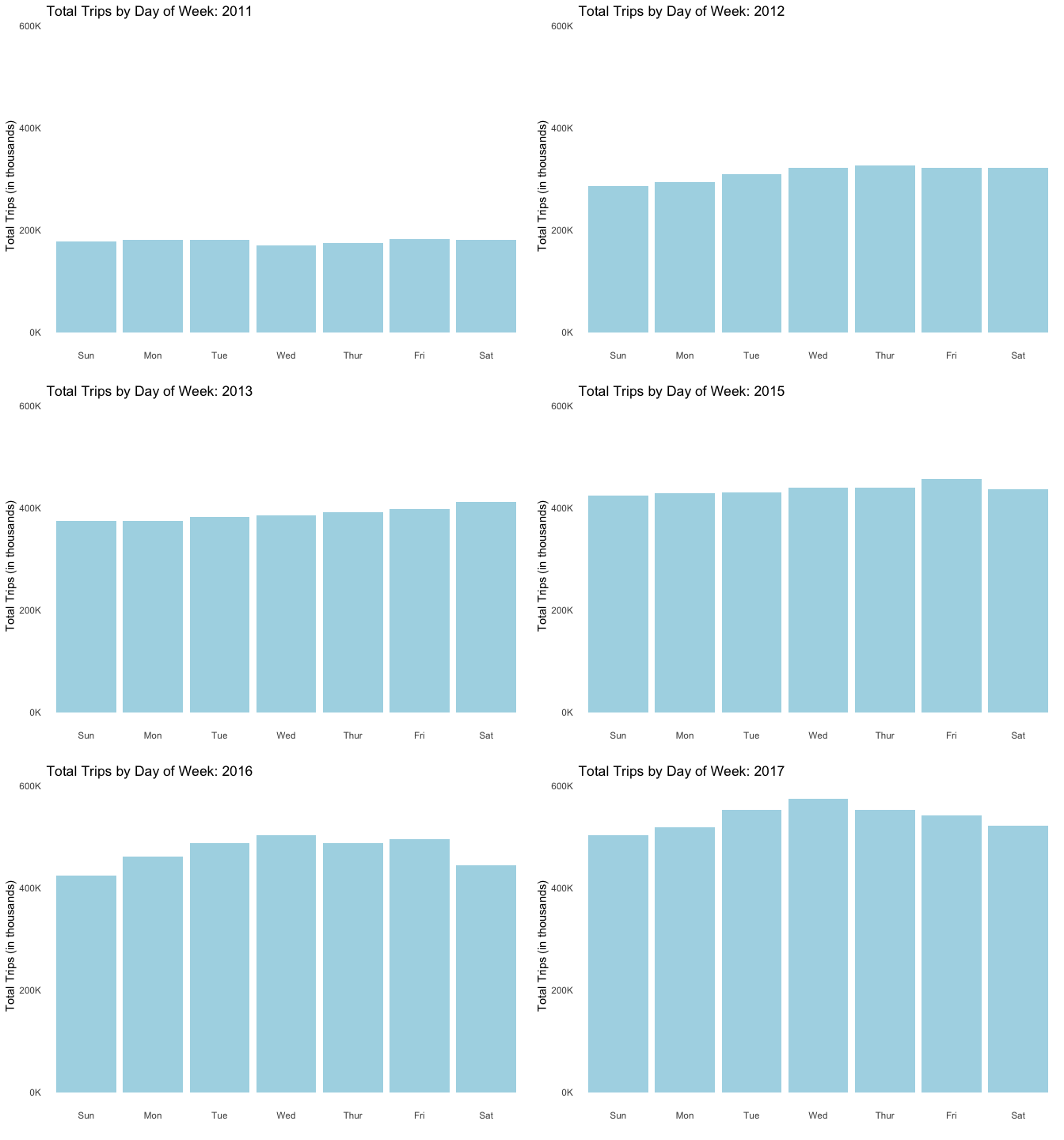
Modeling & Forecasting Methodology
To reiterate, we want to make 30 day ahead trip predictions. We’ll explore several models using (virtually) all of 2011-2016 as training data and an expanding window with a seven day skip period for 2017 as our test data. That was a mouthful. To rephrase, initial model parameters are estimated beginning with all 2011-2016 data. When it comes time to test, the training set is expanded to re-estimate model parameters. Here’s a tabular look at what the training and test sets look like.
It’s fixed origin since the training set always begins at 1/8/2011. We need to skip 1/1/2011 - 1/7/2011 since (spoiler alert) one of the later models uses a lag of 7 of cnt and we want to make model comparisons on the same test sets. We also skip seven days for subsequent training sets since it’d take much more time to run all possible models. For example, instead of making our second training set 1/8/2011 - 1/1/2017 (one day after 12/31/2016) we make it 1/8/2011 - 1/8/2017. So we sidestep having additional training sets 1/8/2011-1/1/2017, 1/8/2011-1/2/2017, … , 1/8/2011-1/7/2017. Test sets are always 30 days long. In total we have 42 training and test sets, created using the createTimeSlices function in the caret package.
The RMSE (root mean square error) and RMSLE (root mean square log error) is used to evaluate models. These metrics are different from each other in that RMSLE penalizes underestimates more stronger than overestimates, whereas RMSE sees both equally. However, both are used since some models have drastically lower RMSEs but almost identical RMSLEs. In a bike share context it’s logical to view underestimates more harshly than overestimates, that’s why RMSLE is considered in this analysis alongside RMSE.
After the 42 RMSE and RMSLE values are calculated from a model we take the median of RMSE since a couple “bad” forecasts can quite skewer the true performance of our model, giving a false impression. We’ll use the mean of the RMSLEs since the RMSLE doesn’t suffer from that skewering.
library(caret)
# use 2011-2016 for fitting model parameters; 2017 testing
bikes_train <- bikes %>% filter(between(TripDate, "2011/01/08", "2016/12/31"))
bikes_test <- bikes %>% filter(between(TripDate, "2017/01/01", "2017/12/31"))

bikes_adj <- bikes[8:2553, ]
# create training and test splits
bike_splits <- createTimeSlices(bikes_adj$cnt,
                                initialWindow = 2181, # row number of 12/31/2016
                                horizon = 30,
                                fixedWindow = F,
                                skip=7)
Model 2: Gradient Boosted Regression Trees
All the models thus far considered only linear relationships. Tree-based methods like random forests and gradient boosted machines are non-parametric, exploiting non-linearities to creating custom if-then statements or rules for prediction (or classification) tasks. Gradient boosting trees are applied here to unlock further predictive accuracy.
Since boosting uses tree-based methods, it does not automatically account for time series data. This is important since each tree in boosting is created by bootstrapping the training data in a random fashion. Order matters in time series, so random sampling can destruct time dependencies within data. Another issue arising from standard tree methods is failure to extrapolate increasing (or decreasing) trend for forecasting tasks. The final predictions from each tree during model building are averages of the response variable from the training set. The test set, by contrast, will include values of the response variable outside the range of the training set. This leads to systematically underpredicting test set data if there’s positive trend, or systematically overpredicting if there’s negative trend. Check this Medium post for a visual example.
Our data has clear positive trend (see Overall Daily Ridership) section). To remedy the issues of extrapolation, the response variable is detrended using first-order differencing on the cnt variable (which is called dif1). The model and it’s predictions are based on the dif1, but the final predictions are back transformed to the original scale using the following formula:
\(PredictedOriginal_{t+1} = PredictedDiff_{t+1} + Actual_t\)
In other words, tomorrow’s predicted ridership (on the original scale) is the sum of tomorrow’s predicted difference and today’s actual ridership. To remedy time-dependency issues, we’ll use lagged values of dif1. Using a lag of 7 is the equivalent of looking back over the last week (seven days) of ridership numbers to form future predictions. Using any other lag didn’t improve forecast accuracies. Like Model 2 other predictors like temperature and windspeed are included, except Time since `cnt is detrended. This model also includes first-differenced values of temperature; hence, we look at both a given day’s temperature and the temperature difference between that day and the previous day.
# new dataframe that includes differenced and lagged values of cnt
b2 <- bikes %>%
  select(cnt, weekday, mnth, holiday, temp, hum, windspeed, prec, snow, TripDate) %>%
  mutate(dif1 = c(NA, diff(cnt,1)),
         lag1 = lag(dif1),
         lag2 = lag(dif1, 2),
         lag3 = lag(dif1, 3),
         lag4 = lag(dif1, 4),
         lag5 = lag(dif1, 5),
         lag6 = lag(dif1, 6),
         lag7 = lag(dif1, 7),
         dif_temp = c(NA, diff(temp,1))
  ) %>%
  filter(complete.cases(.))

# rolling window construction
bike_splits2 <- createTimeSlices(b2$cnt,
                                 initialWindow = 2180, # row number of 12/31/2016
                                 horizon = 30,
                                 fixedWindow = F,
                                 skip=7)
library(gbm) # used for gradient boosting trees
n_mods <- length(bike_splits2$train)
rmsle_boost <- c() # store each RMSLE here
rmse_boost<- c() # store each RMSE here
smape_boost <- c() #store each SMAPE here
# for each of the 42 train/test sets

set.seed(100)
for(i in 1:n_mods){
  # this is where the original data and (differenced) predictions will be stored
  # will be reinitialized for each training iteration
  mod_df <- NULL
  rows_train <- bike_splits2$train[[i]]
  rows_test <- bike_splits2$test[[i]]
  mod_df <- b2[c(rows_train, rows_test), ] # dataframe containing train and test values
  boost.bikes=gbm(dif1 ~ .-cnt-TripDate,
                  data=mod_df[rows_train, ],
                  distribution="gaussian", n.trees=5000, interaction.depth=2)
  bike.boost.pred=predict(boost.bikes,newdata=mod_df[rows_test, ], n.trees=5000)
  mod_df <- mod_df %>%
    mutate(Preds = c(boost.bikes$fit, bike.boost.pred))

  # store back-transformed predictions here
  bike_trans <- c()
  for (i in rows_test){
    pred <- mod_df[i, "Preds"] + mod_df[i-1, "cnt"]
    # make any negative predictions be 0
    if (pred < 0) {pred <- 0}
    bike_trans <- append(bike_trans, pred)
  }
  #calculate RMSE
  err_rmse <- Metrics::rmse(mod_df[rows_test, "cnt"], bike_trans)
  rmse_boost <- append(rmse_boost, err_rmse)
  # calculate RMSLE
  err_rmsle <- Metrics::rmsle(mod_df[rows_test, "cnt"], bike_trans)
  rmsle_boost <- append(rmsle_boost, err_rmsle)
  # calculate SMAPE
  err_smape <- Metrics::smape(mod_df[rows_test, "cnt"], bike_trans)
  smape_boost <- append(smape_boost, err_smape)
}
Model 2 Results
This model significantly outperforms Model 1, further reducing the median RMSE from 2302 to 1642. Median accuracy is 87%. As evidenced in the mean RMSLE underpredictions are reduced, dropping from 0.269 to 0.2.
# Median GBM RMSE
paste0("Median RMSE: ", round(median(rmse_boost),3))
[1] "Median RMSE: 1642.325"# Mean GBM RMSLE
paste0("Mean RMSLE: ", round(mean(rmsle_boost),3))[1] "Mean RMSLE: 0.2"# Median GBM SMAPE
paste0("Median SMAPE: ", round(median(smape_boost), 2))[1] "Median SMAPE: 0.13"Model 3: A Naive Model – The Baseline
Finally, we fit a baseline model that simply uses predicts next-day ridership to be that of the current day. Building complex models like the first two above doesn’t give us an idea of how much better they perform relative to simpler alternatives. Simple (naive) models often perform well, especially on financial data. Our naive serves a baseline to compare Model 1 and 2. If the naive performs closely to first two, the naive model should be preferred.
The naive model doesn’t require training and test sets, but to compare its performance with the other two models, forecasts are made only on the test set dates from the the first two models. We want all models to be compared on the same data.
# include lag 1 of cnt variable
b3 <- b2 %>% mutate(cnt_1 = lag(cnt)) %>% filter(complete.cases(.))
# time slices are the same as in model 2
# use the test indices
rmsle_naive <- c()
smape_naive <- c()
rmse_naive <- c()
for (i in 1:n_mods) {
  indices <- bike_splits2$test[[i]]
  actual <- b3[indices, "cnt"]
  naive_preds <- b3[indices, "cnt_1"]
  rmsle_naive <- append(rmsle_naive, Metrics::rmsle(actual, naive_preds))
  smape_naive <- append(smape_naive, Metrics::smape(actual, naive_preds))
  rmse_naive <- append(rmse_naive, Metrics::rmse(actual, naive_preds))
  }

# Median Naive RMSE
paste0("Median RMSE: ", round(median(rmse_naive),3))
[1] "Median RMSE: 2715.094"# Mean Naive RMSLE
paste0("Mean RMSLE: ", round(mean(rmsle_naive),3))[1] "Mean RMSLE: 0.338"# Median Naive SMAPE
paste0("Median SMAPE: ", round(median(smape_naive), 2))[1] "Median SMAPE: 0.23"The naive model fares rather poorly compared to the other two models on all three performance metrics.
Further Research
This analysis focuses on overall ridership numbers regardless of membership type (casual or registered). To predict revenue by membership type we could calculate the proportion of persons belonging to each category from historical data (say, from 2016) as an estimate. Future research can involve forecasting registered and casual ridership numbers separately, combining their forecasts for predicted overall ridership. This in itself still wouldn’t help determine revenue by membership type since memberships are broken down by five different plan types not provided in the dataset, though CB officials would theoretically have such information.
Other research can involve station-level forecasting and use of other model techniques like neural networks.
Conclusion
We examine three competing forecasting models for 30-day ahead bike share ridership for Washington DC’s Capital BikeShare program, the best model being gradient boosted regression trees. It also improves on the best previous research by reducing the number of variables used for regression, with only 8 unique variables are used here compared to 17 by Wang et al. This work can serve as a starting point for refining forecast accuracy at the station level.
Comments on Model Performance
Each model and its performance in the following table. Gradient boosting affords the highest accuracies on all performance metrics but is the least interpretable since each tree in gradient boosting is different, and 5000 were used in each training iteration! Volatility in daily trip numbers means relying purely on calendar and weather variables may not be sufficient for attaining higher accuracies (or lower RMSEs). For instance (as mentioned earlier) the annual National Cherry Blossom Festival is not consistent year to year, and ridership on those days isn’t easily predicted. The volatility can be seen in the numerous ridership dips in 2017, presented in the plot below. Inclusion of other variables mentioned in the Literature Review may help improve forecasts and could be used in future research.